Random Numbers in Matlab

In the past two years, I have been supervising bachelor degree students for their final projects. Unfortunately, most of the projects were related to time series, forecasting, stochastics process, financial mathematics and many topics related to application to statistics in finance. To be honest, this is not my strong suit. As a result, we struggled when reading and using many statistical techniques especially the one in time series. With this notes, I hope to understand and to keep remember those techniques. Moreover, as I am teaching Time Series Analysis this semester, I believe this post will be very useful for my students.

In this post, I concentrate on how to generate random numbers with certain distributions in Matlab and its application in my time series lecture. I know that we can easily google on how to do these, but as always, it would be very nice to have this ready in my blog. When I forget to do this, I don’t have to google it again and save myself a few minutes.

Generating random numbers and introduction to subplot, histogram, state commands in matlab

To generate random numbers in Matlab with certain distributions, I  need to type

x1 = normrnd(mean,std,[m,n]); %normal distribution
x2 = binornd(N,p,[m,n]); %binomial distribution
x3 = exprnd(lambda,[m,n]); %exponential distribution
x4 = gamrnd(a,b,[m,n]); %Gamma distribution
x5 = rand(m,n); %uniform distribution
x6 = poissrnd(lambda,[m,n]); %Poisson distribution

The commands above returns an m x n matrix containing pseudorandom values drawn from normal, binomial, exponential, gamma, uniform and Poisson distributions respectively. Some usefull commands related to random number generator in Matlab are

subplot(2,2,1) %top left figure
hist(x1) %histogram of normal random numbers
subplot(2,2,2) %top right figure
hist(x2) %histogram of binomial random numbers
subplot(2,2,3) %bottom left figure
hist(x3) %histogram of exponential random numbers
subplot(2,2,4) %bottom right figure
hist(x4) %histogram of Gamma random numbers

The above commands return histograms of random numbers generated by the previous commands.  The output of those commands is the following figure.

Another useful command regarding random number generators is the ‘state’ option. This is very usefull if we want to repeat our computation that involves random number. The following code will help us understand how to use the state command.

clc;
clear;
theta = -0.8;
phi = 0.9;
mu = 0;
sigma = 0.1;
%-----generating random numbers-------------------------
normrnd('state',100);
e = normrnd(mu,sigma,[100 1]);
%-----generating MA(1) and AR(1) process----------------
y(1) = 0;
z(1) = 1;
for i = 2:length(e)
y(i) = e(i) - theta*e(i-1);
z(i) = phi*z(i-1) + e(i);
end
%-----plotting MA(1) and AR(1) process----------------
subplot(2,1,1)
plot(y,'r*-')
subplot(2,1,2)
plot(z,'b*-')

Using the above command, especially when we write the ‘ state’ option in line 8, it allows us to repeat our computation later. We can show the result of our computation tomorrow exactly the same as our computation we conduct today, even though our code involves a random number.  The result of the above command is plotted in the following figure.

Plotting the auto correlation function and introduction to bar command

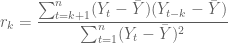
In time series analysis, when we have a time series, it is common to plot the sample auto correlation function (ACF) to be compared to time series models we have in the textbooks. The thing is today, our students now rely heavily on statistical softwares to plot the ACF so that they forget how to plot it in the beginning.  Recall that the sample ACF of the observed series is defined as

(1)——–

The following code shows a MATLAB code that will plot the ACF of both time series generated by the code above.

sumY = 0;
sumZ = 0;
for i = 1:length(y)
sumY = sumY + y(i);
sumZ = sumZ + z(i);
end
ybar = sumY/length(y);
zbar = sumZ/length(z);
sum2Y = 0;
sum2Z = 0;
for i = 1:length(y)
sum2Y = sum2Y + (y(i)-ybar)^2;
sum2Z = sum2Z + (z(i)-zbar)^2;
end
for k = 1:length(y)
sum3Y = 0;
sum3Z = 0;
for t = k+1 : length(y)
sum3Y = sum3Y + (y(t)-ybar)*(y(t-k)-ybar);
sum3Z = sum3Z + (z(t)-zbar)*(z(t-k)-zbar);
end
ry(k) = sum3Y/sum2Y;
rz(k) = sum3Z/sum2Z;
end
subplot(2,1,1);
bar(ry);
subplot(2,1,2);
bar(rz);

The last two commands above will plot the ACF of time series and in the bar style as it is always for the ACF, as shown in the following figure.

 

 

It doesn’t show, really, the supposed to be acf of MA(1) (above) and AR(1) (below) process. Perhaps this is I have not learned  the sample acf measurement (1).

How to export/import data between Matlab and Excell

Finally, we are going to write a code in Matlab on how to export or import data to/from Excell in Matlab. Again, this is to save myself a few minutes rather than googling it around the internet.

%--------------write data to excell-----------------------
y = transpose(y);
z = transpose(z);
filename = 'ma_ar_data.xlsx';
xlswrite(filename,y,1,'A1');
xlswrite(filename,z,1,'B1');
%-------------read data from excell----------------------
filename = 'ma_ar_data.xlsx';
sheet = 1;
xlRange = 'A1:A100';
dataY = xlsread(filename, sheet, xlRange);

The transpose command above puts the variable generated before to be a column vector.

Conclusion

In this post, I have created various codes so that I am able to remember

• generating random numbers
• using subplot
• using histogram and bar
• exporting/importing data to/from excell
• plotting the ACF